Optimality models
In the last lecture, we said the usual approach of behavior ecology is to decide what the best behavior would be in a particular situation. Then you kind of design the behavior, as you would if you were an engineer. The main tools for doing that are optimality models. Today we’ll discuss what they are and how to do them. First, we’ll talk about optimality models in general, and then we’ll talk about a special class of optimality models that you use when what one animal does depends on what other animals are doing.
What are optimality models?
Optimality models balance the benefits of behaviours with their costs. That’s why they call them “optimality models”; they don’t necessarily find the best thing, but rather find the optimal thing. Also, optimality maodels lay out your logic in a very transparent way, specifically by being quantitative. If you commit yourself to to quantitative arguments about exactly how things should go, then you’ve kind of put your money where your mouth is. You’ve made it very clear what you mean when you say the behavior animal should behave in a particular way. So optimality models avoid lots of kind of fuzzy, vague talk about how animals should behave. We’ll have lots of examples of optimality models in this course, especially in the foraging lecture. But what is really nice about them, and you’ll see, particularly in the foraging lecture, is that they enable you to make quantitative, in other words precise predictions and tests of your hypotheses. Our arguments above surrounding the hypothesis about the zebra tailed lizards or the reddish egret were kind of wooly, because they were just verbal. But if instead you say, this bird should prefer a mussel of this size on average, then it’s a very precise prediction. You then get more effective tests of your hypotheses about why the behavior evolved. So what I’ll do in this lecture is present to you two general approaches to optimality models: first, optimality models for just one individual, and then game theory models, which apply when what one individual does depends on what other individuals do as well. They’re known as game theory models because you’ve actually got a number of individuals in your kind of game and things are playing out in a particular way. That’s all sounds vague at this point, but you’ll understand once I go through these models below.
A simple optimality model
So first of all, let’s talk about simple, optimality models. To do this, I’ll do what I do always, is use a cartoon, a made-up example of a behavior that’s a real behavior, but that I’ve picked not because there’s real tests of it out there, but because it illustrates the point. It has to do with terns. They raise their chicks, they lay their eggs on the ground and raise their chicks there until the chicks are big enough to fly off. When they’re at the nest, they’re on the ground, so they’re very vulnerable to predators like this fox that you see here. The terns dive-bomb the fox to try to get the fox to go away from their nests. This is an interesting behavior that they do. How is it crafted through evolution by natural selection? How should the tern behave? It’s doing a lot of things there, taking a lot of risks. There’s obvious advantages to it. But how exactly would the optimal tern behave? Can we kind of predict what natural selection would favor and predict something about, the “perfect” behavior in this situation? Well, here’s how to do that; how to do an optimality model. There’s three basic steps: define the behavior as a simple decision, define your constraints, and choose your currency. First, you’ve got to define your behavior as a simple “decision”. This is why we talk about decisions in behavioral ecology; even though they’re not conscious actions, we’re just trying to kind of make things simple. The animal could behave this way versus that way, and we’re trying to figure out why they behave this particular way. In this example, there’s lots of things we could do here. We could we could talk about how quick the tern should dive at the fox, how fast its flight should be, how much it should call, how often it should dive, and so on and so forth. But if we try to build all that stuff into our model, we’re not going to get anywhere with our model, because it’s going to be too complex. So we simplify things at the cost of oversimplifying things, perhaps, but at the enormous benefit that problem becomes tractable. So in this case, I’m just going to ask, how close should the tern dive at the fox? Why did I pick that? Because it kind of captures the essence of the problem. If the tern dives too closely at the fox, it’s going to risk getting nailed by the fox, snapped up by the fox. If it doesn’t dive closely enough, then it’s not going to drive the fox away from its nest. Indeed, in all elements of an optimality model, not just the definition of the decision, but also the constraints and currencies and so on, you want to capture the essence of the situation. There’s a real art to that. But you kind of use common sense, your gut feeling, your naturalist knowledge, and, most of all thinking it over, trying things out, and discussing it with others. So that’s that’s what we’re going to do here: How close should the tern dive at the fox. That’s a simple decision.
Now we’ve got to define the constraints: the things that that that the animal’s stuck with, that it can’t do anything about: the problem the animal is faced with having to solve. In this case, given that the closer I do go to the fox, the more likely I am to get grabbed by the fox. That’s just a fact of life; there’s nothing I can do about it; it’s a constraint. Another constraint is that I have to get close to the fox to drive the fox away. There’s nothing I can do about that, either; that’s what makes getting close effective. The problem set by the model is: given those constraints, then how should I behave? To solve this problem, you’ve got to choose a currency: what the animal’s after. What is it trying to maximize? You know that the animal won’t be able to maximize absolutely, because it’s got to strike some kind of balance between benefits and costs. But it should be selected to maximize some kind of currency that ultimately translates into greater survival and reproductive success, greater fitness. The currencies are the immediate things that that the animal is, quote unquote “trying” to maximize, like finding lots of food or getting lots of energy, like our oystercatchers were. Ultimately, whatever it is, it has to translate into greater survival and/or reproductive success. So usually in an optimally model, when you choose a currency, it’s that immediate thing that ultimately translates into greater fitness. In this case, though, because we’re mixing that the chance that the tern will be killed by the fox (survival) with the chances that its young will survive (reproductive success), both of which ultimately end up in greater fitness, we’ll just simplify things and call it fitness. We’ll play around with currencies some more in the foraging lectures, leaving aside further discussion until then. OK, so now we’ve got all the key elements in our optimality model. Now what we’re going to do is write this all out quantitatively. I’m not going to do it in terms of equations; I’m going to do it graphically because what I’m after is a kind of intuitive appreciation of all this.
A tern defends its nest
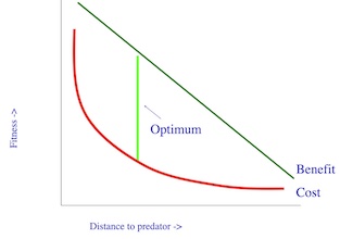
Our optimal mobbing model
A tern’s fitness payoff for defending its nest. The closer it gets to the fox, the better its nesting success (and thus fitness), but as it gets very close, its risk of getting caught by the fox abruptly increases (a big fitness value is subtracted).
Game theory models
OK, that’s an optimality model for one individual. But the fact is that these terns are in colonies. So the attack of the fox is more something like this. So you can see a lot of these terns are being very nasty to us, standing in for the fox. But there’s lots of terns attacking and that changes things quite a lot.
What should the optimal behavior be? The optimum behavior in this case depends on what other individuals are doing, because if you think about it, if somebody else is going close to the fox, then a tern can hold back and still get some benefit, because another tern’s doing all the work for you. So now the optimum behavior might be to hold back a little bit more because others are doing the work. Conversely, if everybody is being chicken about attacking the fox, then that tern is not going to get any protection.
So for this situation and for many situations in the course where we’re dealing with the behavior of lots of individuals all at once, the optimum behavior depends on what other animals are doing. And for that, we use a different technique, which is also a form of optimality models, called “game theory”. It’s called game theory because, basically, we treat the animals as if they’re playing some kind of game with each other. In this case, the game of a pretty serious game, but the game of chasing a fox away from their colony. What the game is meant to show you is the evolutionarily stable strategy, which is the behavior that, once adopted by most members of the population, is likely to be evolutionarily stable - i.e., to persist across generations. It’s often not the optimum behavior for a given individual, but it’s what adaptation by natural selection ends up with, because all these different players are are all trying to optimize their fitness. It explains lots of situations where there’s a balance of different behaviors. So where there is some, you know, fighters versus chicken animals that that hold back but are more sneaky and animals that display loudly for four mates and others that sort of sneak around and kind of find mates that way.
We’ll see lots of examples of game theory as we go through this course. But I must show you the basic outlines of game theory right now, so you’ve got it in your head. The end result of a game theory model is that you you’re after finding the evolutionarily stable strategy, that’s the ESS, a term that will come up a lot in this course. That’s a strategy, which is a behavior or a mix of behaviors, that, once it’s adopted by most members of the population, can’t be beaten by any other strategy in the game? Sounds pretty confusing for now, but you’ll get the idea once we work through a couple examples.
There’s two ways to find the ESS: One way is to look to see where the payoffs are equal, and that’s usually done graphically. I’ll show you an example of that for our mobbing thing in a second. Alternatively, we can imagine if a new strategy could do better. We can do that process graphically, too, or we can use something called a payoff matrix. What I’m going to do in next is go through each of these techniques. First we’ll use the graphical technique for the mobbing example, and then we’ll use another game to introduce the the the idea of a payoff matrix.
Here’s a cartoon example for our tern, a situation where you’ve got the relative fitness on the Y axis, and on the X axis,you’ve got the proportion of a daring phenotype versus a cautious phenotype. So daring versus cautious mobbers on the x axis. So the way the X axis work works is like this down at the top of the x axis. The population consists entirely of cautious mobbers, at the lower end of the x axis, They’re all daring mobbers. And then there’s varying proportions running in the middle. So let’s imagine what the fitness curves might look like. Of daring and cautious mobbers with this game theory model with here’s a reasonable curve for cautious mobbers. If the whole population consists of daring mobbers. So we’re over here on the left end of the x axis, then everybody’s doing. And your cautious mobber, then everybody’s doing the work for you. You just hang back and let them all take the risk with a fox. They get nabbed up. They have may have lousy fitness, but you have great fitness because they’re doing all the work for you. You suffer none of none of the costs. None of the risks of getting shot by the fox. But imagine if everybody’s cautious, a cautious mobber. Everybody in the population, then the there might be only one or two daring mobbers in the population because the population is just about all cautious mobbers. And that means that the fox is just going through the colony, chowing down on on all these nests. So all of your cautious mobbers are having lousy success, whereas daring mobsters. If we draw the curve for daring mobbers, they do great when the population is all all cautious and they do lousy when they’re all daring and they’re all suffering the cost of of the fox. And what happens in between? Well, and here’s the tricky thing. And you’re gonna have to do this on your own to kind of work your head around it. But imagine, let’s start at the left end of the X axis and imagine a population, all of daring members. If that’s the situation, then cautious mobbers are going to have a great fitness. And what that means because of what fitness means is that that’s going to increase over evolutionary time. That’s going to increase the proportion of cautious mobbers in the population. So the population is going to move to the right on this. Conversely, if we started at this end, if the whole population is cautious, then the daring mobbers are going to do much better than the cautious mobbers and that’s going to shift the population this way. And so over evolutionary time, you can imagine that the population is going to go wobble, wobble, wobble back and forth and end up right here where this is going to be a sort of stable equilibrium. And that’s the evolutionary stable strategy. So that’s the solution of our game theory model. Okay, so that’s that’s one way to do a game theory model. Another way is the payoff matrix. And I’ll show you that just very briefly. We’re going to fiddle with it more in our Thursday exercise. Imagine it’s funny cartoon, sort of funny, not all that funny. A world with which they’re playing rock, paper, scissors and. And they’re all playing rock. Then they play this game. And, oh, everybody’s tired all the time. Imagine if that population were invaded by individuals who played just paper. They would quickly overwhelm the rock population. But if we have a population of rock, paper, scissors, then things get more complex and we can express this with what’s called a payoff matrix. And you’ll often see game theory models presented this way. So that’s why I’ve come up with this example to just show you the basic features of a payoff matrix. So we have an actor and a reactor. You can set this up in various ways, but that’s often how they’re set up. So in this cell here in the table, rock is playing rock. What happens when rock plays rock? What have. Is when the actor plays Rock Against a reactor who is also playing rock, what will the reproductive success of the actor be? Well, you end up being. It ends up being a draw. But if rock pays against paper, then rock the actor loses. And so on through the table. I’ll just let you work it out on your own. If you stare long enough at this payoff matrix, what you want to figure out is what’s the winning strategy? And sometimes it won’t be necessarily just one thing. But sometimes you can look at this payoff matrix and see that one strategy is going to win. And that’s gonna be the evolutionarily stable strategy. And in this case, that’s the case. You think about it. Paper is going to sweep the population and we can play around with that. And we will. On Thursday. Now, the interesting thing with this payoff matrix is that when you throw scissors into the mix, then everybody has pretty much equal reproductive success. But things … so, So what you would expect in this population is you’d expect roughly equal proportions of rock, paper, scissors for this particular game. Things aren’t that simple and we’ll find that on Thursday. But for most cases, when you look at the payoff matrix and you can see that that there is a balance of behaviors favored, then that’s the evolutionary stable strategy, is to play those strategies with some sort of particular probability. So that’s a quick introduction to game theory and to optimality models. And I’ll leave it there for now.